“Errors are beautiful and Gaussian”-Really?

Soumya Sengupta

Gaussian or Normal Distribution is the most common of all the probability distributions in the sense that the heights of the boys in a classroom, the errors in any experiments, or the probability of acceptance of your proposal (in your company or in love affairs) all follow the Gaussian distribution. De Moivre first reported the Gaussian distribution, and Sir Gauss worked for its development.

The Gaussian distribution function has the following mathematical form,

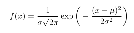
where,

1. µ is the mean value or the expectation value of the probability distribution i.e. the probability of finding the variable x in this distribution is maximum at µ
2. σ is the standard deviation of the distribution.

Here in figure 1, you can see the bell-shaped structure of the Gaussian distribution function. The probability is clearly maximum at µ = 2.

Now I will show practically how we can get Gaussian distribution in an experiment:

Suppose, I toss an unbiased coin (For an unbiased coin the probability of getting” Head” or” Tail” is exactly the same) N number of times. As the coin is unbiased, we expect there is a high probability of getting an equal number of head and tail, provided N is large. How large? Suppose N=10. Then obviously the probability of getting an equal number of heads and tails is very less. Now if we plot it in a graph and check how many heads or tails are there for N number of tosses, let’s assign ”+1” with head and ”-1” with a tail. So, after N number of tosses if we add all these assigned values then the sum should be equal to zero (as the probability of getting Head and Tail is equal). As we expect the sum of this assigned value is zero so technically the mean or expectation value for this experiment is zero.

Now if we perform this same experiment for M number of coins then the sum will not be always equal to zero (obviously, right?). So, what will be the minimum and maximum value of this sum for N=10 number of tosses? If all outcomes are ’tail’ then the sum S=-10 (which is minimum) and when all are ’head’ then S=10 (maximum). Therefore, in one sentence,

For N number of tosses, the minimum value of the sum of assigned values is -N and the maximum is N while the assigned values are ±1.

Now we can think about M which is the number of coins to do the experiment. If we do this tossing with really large (how large? Suppose M=10,000) number of coins and plot the histogram of those summed values we will get the following graphs.

Figure 2: Histogram plot of the sum of assigned values of the coin-tossing experiment at N=10 and M=10,000. See, it takes a Gaussian shape.

From Figure (2a) it is clear that when M is large (10,000) then the histogram looks like a gaussian. But the bar-like structure is due to the integer sums. If we replace that “+1” or “-1” steps by some random numbers between -1 to 1 then the diagram will change its shape as Figure (2b). In Figure (2b) we can observe that the maximum and minimum of the summed values changes from ±N. This is because the assigned random numbers are in between -1 and 1.

Let’s progress further in this experiment. We can now fix the number of coins (i.e. M=10,000) and increase the value of N from 10 to 100, 1000, and so on. Then the histogram will change as shown in figure 3.

Thus, by increasing the number of tossing in this experiment we will get sharper and sharper Gaussian.

Now, it’s time to conclude this experiment and give some predictions with logical intuition.

1. If we increase the number of tosses (i.e. N) with a fixed number of coins (i.e. M fixed), then the sharpness of the histogram will increase. So, if we increase N infinitely the Gaussian will become a delta function (Ohh really! You can think about it.) (Here the delta function distribution means that the probability is fixed at a particular point.)
2. One more thing to note is that the height of the Gaussian is directly proportional to N (i.e. number of tossing) while the flatness is inversely proportional to N for constant M.
3. Whatever be the value of M (i.e. number of coins) or N, the shape of the Gaussian remains the same. Look how beautiful the errors are! They are always symmetric on both sides from the mean, irrespective of where the mean is.

In this note, I have discussed a little about the starting point of a Gaussian distribution. You can think more, play more, and have more fun.

About the author
Soumya Sengupta is a Senior Research Fellow at IIA and he works on modelling of Exoplanet atmosphere.